When one wants to keep time, or needs an accurate frequency standard, then atomic clocks
are the way to go.
Back in the days, one had the choice between three types of atomic clocks that one could
commercially buy:
Rubidium vapor cell standards
Caesium beam standards
Hydrogen masers
Back then, the choice was pretty simple and straightforward given the constraints one had.
Today, we have a plethora of potential atomic clocks one can buy with quite a few more
being in development.
So the question which one to use becomes more difficult.
I will try to give here a (not so) short summary of how the different types work, what their
advantages and disadvantages are, and how to choose based on these.
It is kind of customary to sort atomic clocks based on the atomic species they use.
But the same species can be used for different types of atomic clocks.
Or the same type of atomic clock can be built with different atomic species.
E.g., beam standards have mostly been built using caesium, but it is equally possible
to build them using rubidium, there have even been attempts to build one using hydrogen.
Thus I will sort the atomic clocks by their types, where type usually means how the
atoms are moving or held in place and how they are probed.
I will also use “atomic clock” and “frequency standard” interchangeably.
While this is not correct according to the definitions:
A clock is a precise/stable
frequency source with a counter that can display or measure the passage of time.
A frequency standard is a frequency source that provides an
accurate frequency output to
calibrate other frequency sources.
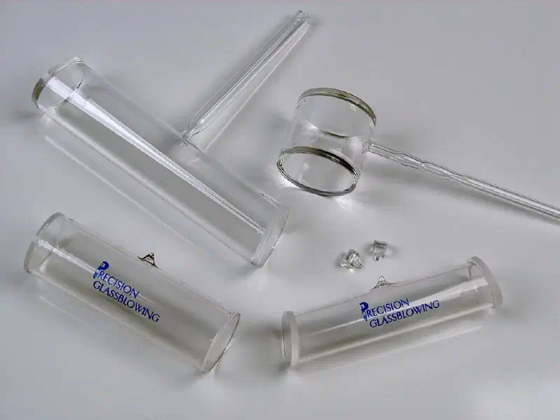
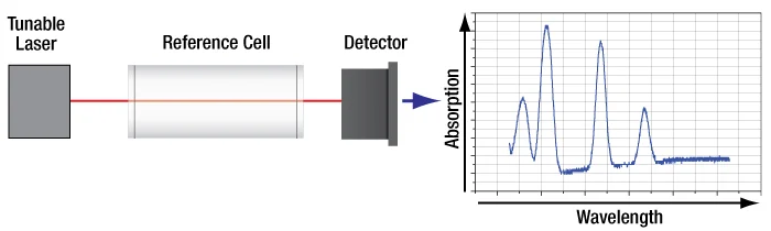
Vapor cells are, at their simplest, just an enclosed tube with two optical windows that
contains some type of substance to be probed.
The probing happens by shining light (usually a monochromatic source like a laser) into
one and detecting what comes out at the other.
While the name implies some kind of vapor in the cell, the amount of vapor is usually
so small that it is not visible to the naked eye.
Or rather, it should not be visible, because then the vapor is so dense that any
probing light gets completely absorbed and there is nothing left to be detect.
Which means only a tiny amount of the substance should be floating around in the cell.
This is achieved by either adding only a small amount of the substance to the cell
or by keeping the cell’s temperature way below the substance’s boiling point.
The latter approach is used with vapor cells in atomic clocks.
E.g., rubidium has a boiling point of about 688°C (and a melting point of 40°C).
Typical temperatures for rubidium vapor cells are between 50°C and 70°C.
At these temperatures already enough rubidium evaporates to make the rubidium
optically dense in short vapor cells, i.e., at the correct wavelength, all light gets absorbed
and adding more vapor or using a longer cell does not increase the signal to noise ratio (SNR) anymore.
Another method used for detection is fluorescence. I.e. not the absorption of the light sent in is
detected, but rather the fluorescence that the light causes, either at the same or a different
wavelength.
When the fluorescence happens at a different wavelength, this allows for filtering of the light
that gets scattered without interacting with any atoms and thus a higher SNR can be achieved,
which in turn leads to a more robust detection of the light-atom interaction.
This is especially popular in two-photon absorption schemes.
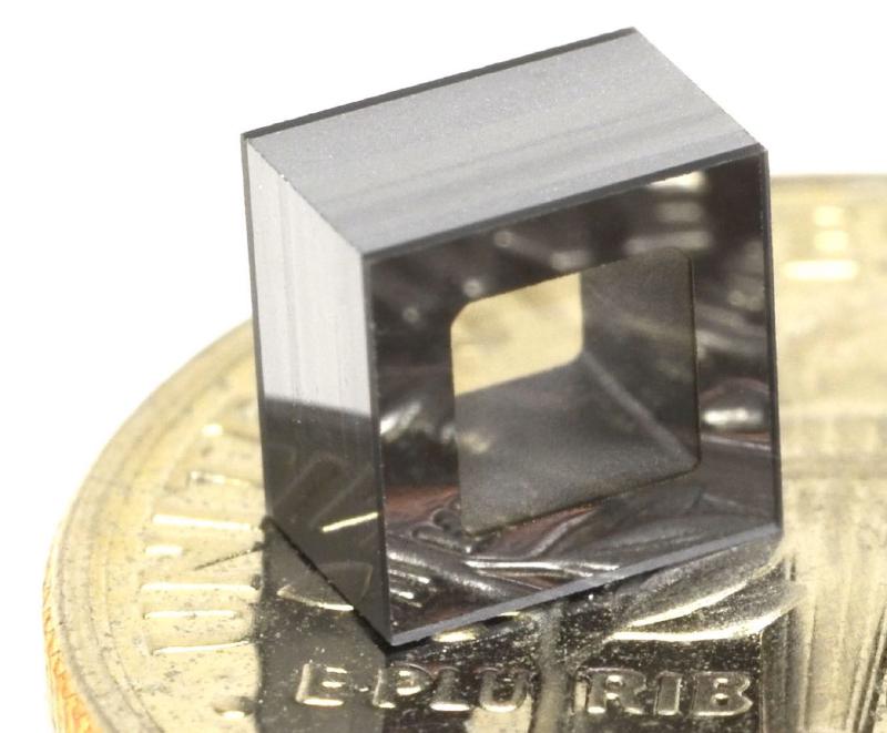
While the vast majority of vapor cells are manufactured using glass, that does not need
to be the case.
In recent years, micro-fabricated cells based on anodic bonding
of glass to silicon wafers have gained popularity.
This allows for tiny cells, just 1-2mm of size, and thus an extreme miniaturization of the
whole system.
The most basic form of a vapor cell based standard is what we today call the dual or double resonance
vapor cell clock (in contrast to the coherent population trapping clocks that come later), which uses
two sources resonant with the atomic species, one light source and a microwave source.
In the 1950s, people realized that they could use a lamp based on rubidium 87 and filter it
using a vapor cell containing rubidium 85 and due, to a fluke of nature, it would leave a spectral
line that would pump Rubidium 87 into a specific hyperfine state (see also
“A History of the Rubidium Frequency Standard
by William Riley).
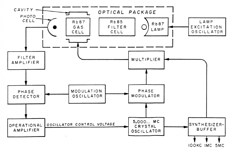
This was first made into a commercial product by Varian in the early 1960s, the Varian V4700 whose
block diagram is depicted above.
The rubidium 87 lamp on the top-right shines on the Rb87 vapor cell on the top-left.
The vapor cell is placed in microwave cavity and gets a signal of 6.8 GHz, which changes
the amount of light absorbed by the cell, depending on whether the signal is exactly on resonance
or not.
The amount of light gets detected by a photo cell, whose signal is then fed into a feedback circuit
that controls a crystal oscillator (OCXO).
A more detailed explanation can be found in William Riley’s “Rubidium Frequency Standard Primer”.
The advantage of this approach is its simplicity and use of very robust components.
The lamp is a simple vapor discharge lamp, the vapor cell, once fabricated, barely
changes its properties.
Which allows these standards to be produced quite cheaply and sell for as low as €1000.
The disadvantage is that they are not that great in terms of stability.
The low-cost “telecom grade” rubidium standards deliver about \( 10^{-11}/\sqrt{\tau} \)
short-term stability, but bottom out at 5 to 10 parts in \(10^{-13}\) before the
frequency drift due to temperature changes starts to show up.
The better ones bottom out at about \(10^{-13}\) and stay there for \(\tau\) up to
\(10^4\) to \(10^5\) seconds.
In the early 2000s academia switched to using lasers instead of a gas discharge lamp,
which improved stability significantly and allowed to use
Ramsey interrogation, which
improved stability even further.
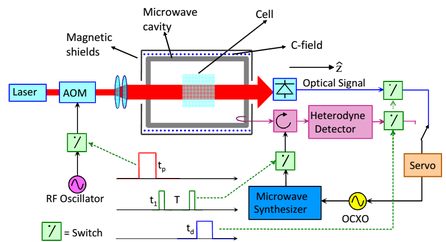
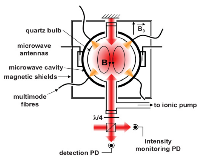
Today, state of the art systems, like the pulsed optical pumping (POP) clocks
(see picture above) developed at
University of Neuchâtel
and INRIM reach short-term stabilities
of \(1\text{-}2 \cdot 10^{-13}/\sqrt{\tau} \) and a flicker frequency floor
of \(7\cdot 10^{-15}\)
Unfortunately, these designs have so far not been commercialized.
I guess the space between the telecom grade Rb vapor cell standards and the
caesium beam standards does not leave enough room for an alternative design
with better short-term stability than either of those, but worse long-term
stability than caesium beam standards.
One disadvantage of dual resonance vapor cells is the need for a resonant microwave cavity
for the hyperfine splitting frequency (e.g., 6.8GHz for rubidium 87), which can be quite large.
While there are tricks to make those smaller (like the
magnetron type resonator and the
micro loop-gap resonator developed in Neuchâtel),
there is an ultimate limit how small these can get, as they still need to work with microwaves
of a specific wavelength.
This is where coherent population trapping (CPT) or electromagnetically induced transparency (EIT)
comes to the rescue.
While the phenomenon has long been known, it was only introduced as a means to build a microwave
atomic clock by Cyr, Têtu, and Breton in 1993.
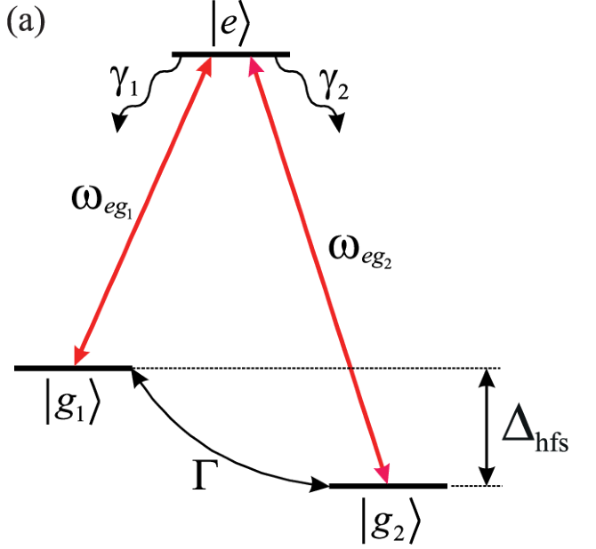
CPT works on the principle that if you have an atom with a three level system, where
you can optically excite it using two different wavelengths (or frequencies) such that
the processes share one level ( \(\omega_{eg1}\) and \(\omega_{eg2}\) with \( |e\rangle\)
as shared level in the above diagram), with the transition of the other two levels
( \(|g_1\rangle \) and \(|g_2\rangle \) ) being “forbidden”.
Then exciting both transitions \(\omega_{eg1}\) and \(\omega_{eg2}\) leads to a cancellation,
which means neither transition happens.
This “dark state” (so called because there is no fluorescence) is very narrow, about as wide
as the hyperfine splitting itself, thus allowing to lock onto the hyperfine splitting without
the need for a microwave cavity.
I.e., the vapor cell can now be almost arbitrarily small.
The tiny vapor cells mentioned above were all designed to be used with CPT.
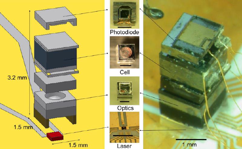
And this make for some really tiny atomic clocks, as NIST demonstrated with their
chip-scale atomic clock (CSAC).
The CSAC was later commercialized by Microchip as CSAC SA45 in a 40×35×11mm package, which was a huge success.
But this miniaturization comes at a cost: the short and long-term stability of the CSAC is much worse than
that of a telecom grade rubidium vapor cell.
If you are being mean, you’d call it an expensive OCXO.
But, the big advantage of the CSAC is achieving better than OCXO stability at a 1/10th of the power consumption,
which is for many applications a game changer.
Interestingly, the Swiss company Spectratime (now part of French Safran) was able to miniaturize a
dual resonance rubidium vapor cell down to 50×50×20mm, called the
mRO-50, which is only slightly larger than
the CSAC and is a standard OCXO form factor.
They achieve better short and long-term stability too.
The next group of atomic clocks are beam and fountain standards, which are probably what most people
think of, when talking about atomic clocks.
The basic operating principle is a bit more complicated than with vapor cell clocks.
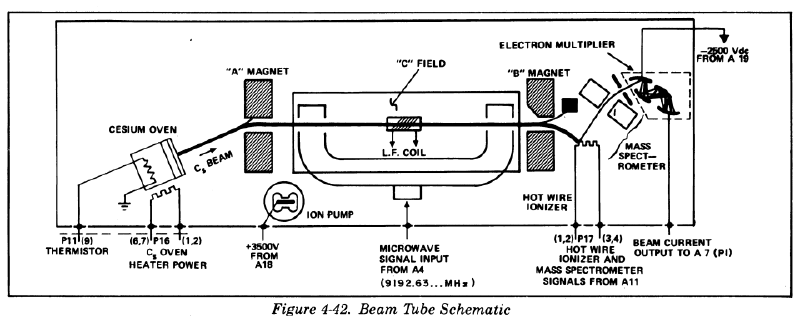
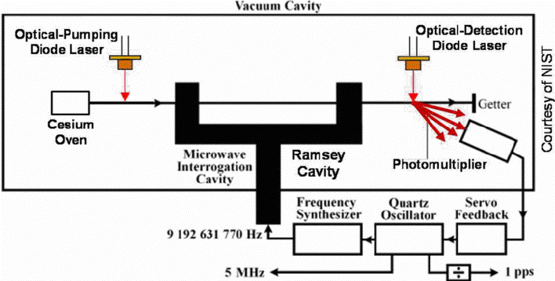
The above diagram is from the HP5061A manual.
The beam tube is a vacuum chamber within which the caesium atoms fly through while being interrogated.
A caesium beam is generated in an oven, a small crucible with a few grams of caesium and a small hole to
direct the atoms flying out into the right direction.
The A and B magnets are basically Stern-Gerlach
selectors to select the atoms in the right hyperfine state.
As the hyperfine state of the atoms is random, and they are equally distributed, this halves the number
of available atoms for interrogation.
The atoms then fly into the interferometry chamber, which has additional magnetic shielding to keep the
magnetic field the atoms see more stable.
There is a slight magnetic field, called the C field, which defines the quantization axis for the interrogation
and allows to slightly shift the frequency of the hyperfine splitting and thus the atomic clock.
The U shaped bow is the microwave chamber.
The U shape is to probe the atoms twice, with a short break in between.
This is the so called Ramsey interrogation,
which results in a narrower peak and thus a more stable clock.
After leaving the interferometry chamber, the atoms fly through another Stern-Gerlach selector, to
detect how many atoms switched their hyperfine state.
The detection itself happens by ionizing the atoms and detecting the ions and electrons generated.
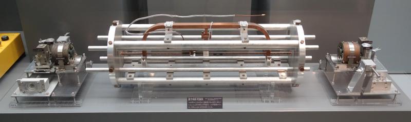
A nice and clean build of such a caesium beam standard is the NICT CRL-CS1 frequency standard that was in use
from 1975 to 1993 in Japan.
The A and B magnets have been replaced by multi-pole magnets which simplify alignment of the whole system, as
they only deflect those atoms in the wrong state and thus the atoms in the right state can fly straight.
Most commercial caesium beam standards do not look this clean and spacious, though.
In the early 2000s, with advancements in (commercially available) lasers, a new type of caesium beam standard
appeared: the optically pumped beam standard.
While the use of lasers instead of magnets might seem to complicate things, after all the lasers need to be
locked to the right frequency/wavelength, they allow for a straight flying of the atoms, like with multi-pole
magnets, but without any deflection from misalignment of the magnets at all.
And more importantly, they pump the atoms into the right state, thus making use of all atoms available without
throwing half of them away.
This increases SNR of the signal and thus enhances the frequency stability of the atomic clock.
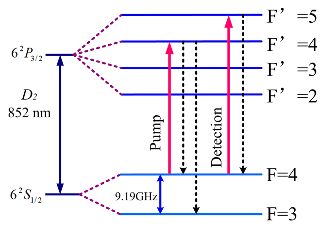
Another advantage is, that one can use two different lasers for pumping and detection.
This allows to use an efficient pumping transition (the \(S_{1/2}, F=4 \rightarrow P_{3/2}, F=4\) transition
in the above diagram), which has a high photon absorption rate, while at the same time a, so called,
cycling transition can be used for detection (\(S_{1/2}, F=4 \rightarrow P_{3/2}, F=5\)), where the electrons
fall back into the \(S_{1/2},F=4\) state with a much higher probability than into the \(S_{1/2},F=3\) state,
the latter transition being forbidden from the \(P_{3/2},F=5\) state, thus getting several hundred of scattered
photons instead of just two, again increasing the SNR.
Optical pumping is not easy, though.
Oscilloquartz released their first optically pumped caesium standard in 2016 after almost a decade of development.
Today there are still only two companies offering optically pumped caesiums, one is Oscilloquartz, the other
is Chengdu Spaceon.
Microchip, the third caesium beam standard manufacturer, has not developed an optically pumped standard so far.
Another way to increase accuracy and stability, is to increase the time separation of the two Ramsey interrogation steps (or \(\pi\)-pulses).
But as the atoms are flying into one direction and you have to use at least a certain temperature
(around 100-500°C) for the oven to get enough atoms, thus giving a fixed speed at which the atoms
come out of the oven, the only way to make the interrogation longer is to make the atoms fly for longer.
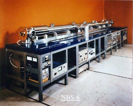
In the case of the NBS-6 caesium beam frequency standard above from the mid 1970s had an interrogation
length of 3.74m, with the overall length being close to 6m.
A small side note: You will see that some companies call their optically pumped caesium beam standard
“optical clocks”, implying they are optical atomic clocks.
But the lasers are only there to pump and detect.
They do not interrogate an optical transition but a microwave transition, making them still microwave atomic clocks.
One big disadvantage of beam standards is, that the flight time cannot be made longer than
a few 10s of milliseconds without making the tube impractically long.
Another is that the atoms’ speed has a distribution depending on their temperature, adding some
hard to control shift to the atomic frequency.
It would be so much better if the atoms were cold, just a few Kelvin, and would fly much slower.
Thus, people came up with the idea of atomic fountains (already way back in the 1950s).
Instead of launching the atoms horizontally, they are launched vertically.
This gives two advantages: First, the atoms can be much slower without the need to make a parabolic bent vacuum tube.
And second, the same microwave cavity can be used for both halves of the Ramsey interrogation, reducing the shifts
due to the cavity geometry.
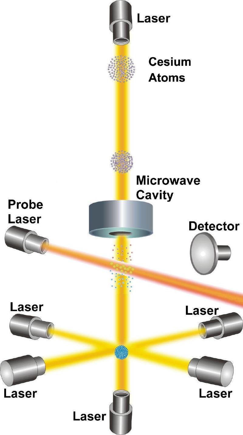
The way this is achieved is by using 6 laser beams at the bottom of the clock to trap the atoms in a
magneto-optical trap (MOT).
There the atoms are cooled down to a few 10s of milli-Kelvin.
Then, by switching off all lasers but the bottom one, the atoms are launched straight up.
On their way up, they pass through the probe laser, which first pumps them into the correct
state, then through the microwave cavity.
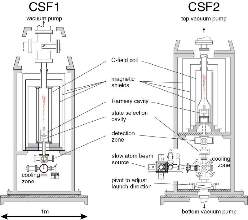
The tube lengths are usually around a meter or so, giving the atoms a flight time of roughly
a second.
On their way down, the fall again through the microwave cavity, getting their second half of the
\(\pi\)-pulse and pass again through the probe laser, which now acts as a detector for the atomic
state.
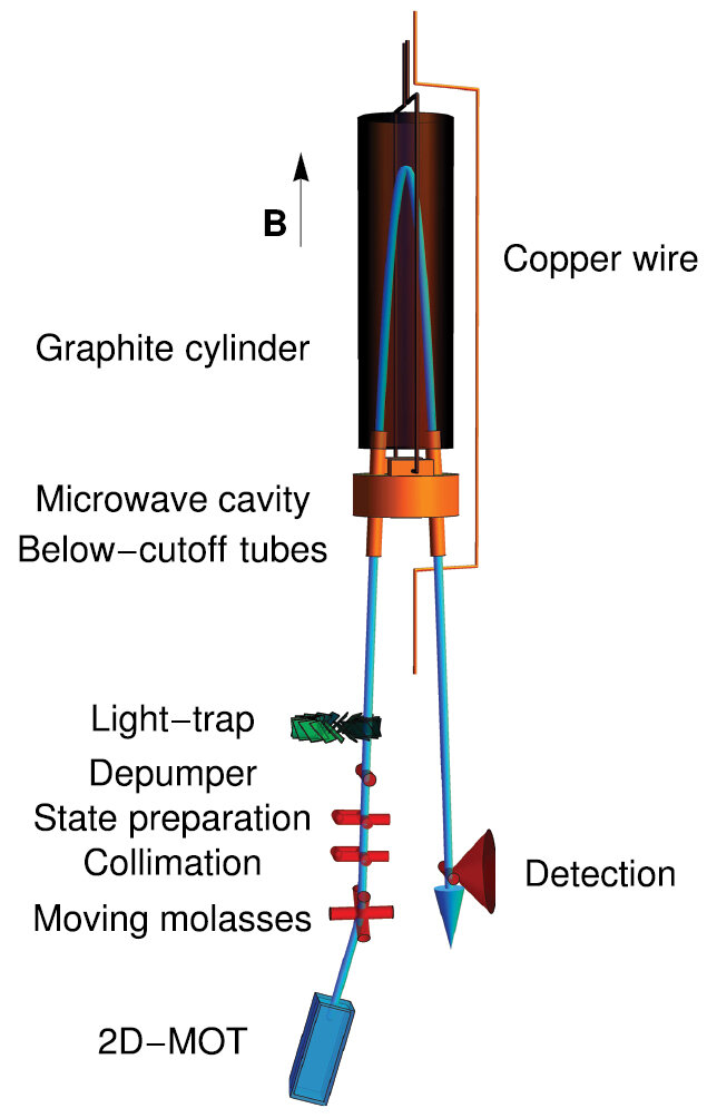
A variant of the atomic fountain is the continuous fountain, pioneered by the Swiss metrological
institute METAS.
In a normal fountain, it is not possible to have multiple atomic packets in flight, as those
on the way up would collide with those on the way down.
Which in turn requires that every collection of atoms in the MOT can only start once
the interrogation of the previous atom packet has finished, giving the fountain clocks a rather long
dead-time, which gives rise to a large uncertainty through the
Dick-effect (Simplified: the time-discrete
interrogation of the atoms leads to a time-discrete sampling of the noise of the local oscillator.
This non-linear effect causes high-frequency noise to be down-converted into the signal band,
increasing the local oscillator’s effective noise more than one would first expect.)
METAS solved this problem by launching the atoms on a slightly angled path, thus separating the up
and down path.
Adding a rotating light trap, which lets the atom packets pass through, but blocks the light from
the MOT, which would otherwise cause frequency shifts.
Of course, using two different paths through the microwave cavity, as with the beam standards,
is the cause of some additional frequency shifts.
But the team at METAS has managed to keep them small and very well controlled, making the FoCS-2 one
of the most accurate caesium beam fountains in existence.
So far, all atomic clocks we have looked at, were passive standards.
Meaning, the interrogation signal has been applied from outside and wasn’t generated by the atoms themselves.
But, we all know that atoms cannot only absorb light (or microwaves), but also emit it.
And this is the idea behind active standards, of which the most prominent (and to my knowledge
the only one that has been actually demonstrated) is the maser.
The name maser does not only sound similar to laser, it bears the same root, being an acronym
for “microwave amplification by stimulated emission of radiation”.
Similarly to a laser, the atoms are pumped into the right state, from which they can fall down
into their ground state, while emitting a (microwave) photon.
Instead of mirrors as in a laser, a resonant microwave cavity is used, to cycle the emitted photons
through the atoms again and again, so they can stimulate the other atoms to emit a photon.
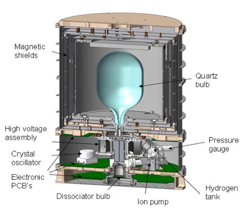
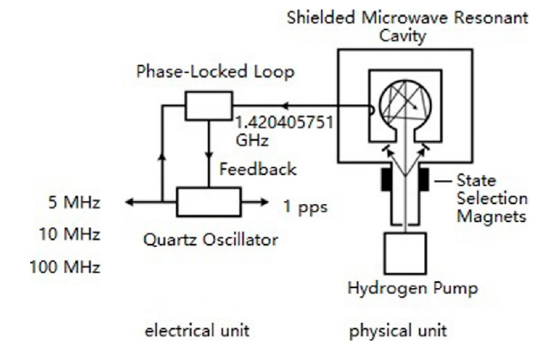
In an active hydrogen maser, the most common type of active maser (and as far as I am aware of, the
only type of active maser commercially sold), the hydrogen is stored in a pressure bottle and passed
through a palladium leak into the chamber.
Then the hydrogen passes through a dissociator (simplified an RF coil that breaks the \(H_2\) molecules
apart into single atoms) which then fly through a multi-pole state selector, before entering the
resonant cavity through a small hole.
To keep the hydrogen atoms in the center of the cavity, there is a small glass bulb within
which the atoms bounce around.
But as each bounce on the glass wall slightly disturbs the hydrogen atom’s electrons and thus
the energy levels, the bulb is coated with PTFE to minimize the shift.
Keeping the atoms within the center of the cavity is important to reduce the shifts that
are associated with the position of the atom within the cavity (due to RF field alignment and phase variations).
The atoms are selected to be in the upper hyperfine split of the ground state ( \(S_{1/2}, F=1, m_f=0 \) )
and when they fall down to the lower state ( \(S_{1/2}, F=0, m_f=0\) ) they emit a photon of 1.420 GHz.
This photon bounces around in the cavity and stimulates the other atoms to also emit a photon, coherent
with the previous one, thus forming a maser.
This signal is coupled out and a quartz crystal oscillator (it used to be a Oscilloquartz BVA 8607)
is locked to this signal and provides the output signals of the clock.
Until recently, these were the best performing atomic clocks for short to mid-term stability.
Achieving an ADEV of below \( 10^{-13} \) at 1 second, going down to a few parts in \( 10^{-15} \)
at one day.
Beyond one day, the drift, mostly due to wall collision and cavity pulling, results in a worse ADEV.
But, the drift behaviour is generally well enough behaved, that it can just be corrected as a linear
or quadratic term and only needs recalibration once a week.
While these days, optical atomic clocks are beating active hydrogen masers in terms of performance, they
are not at the superb reliability that hydrogen masers achieve.
The biggest technological difficulty of active hydrogen masers is that the atoms themselves provide the
oscillation power.
This results in a very weak signal of only a few pW, which makes detection difficult.
It also necessitates that the cavity has a very high quality factor, in order to minimize losses.
This makes it difficult to build compact cavities (which have higher losses) to shrink the size of
active hydrogen masers.
In a passive hydrogen maser, this is solved by generating the 1.420 GHz signal and probing the absorption
of the atoms in the cavity, just like with the vapor cell and beam standards mentioned above.
Because this probing doesn’t require the detection of a very weak signal, the cavity does not need
to have as high a quality factor as with active hydrogen masers.
This allows to use high \(\epsilon_r\) materials (e.g. alumina/sapphire) and more lossy higher order
cavity modes to shrink the size of the cavity.
Of course, this change in mode and shrinking of the cavity comes with a penalty and the short-term
stability of passive hydrogen masers is about an order of magnitude worse than that of active hydrogen masers.
While not a commercially available atomic clock, this is, in my opinion, too cool to not mention: the solid state maser.
The hydrogen maser uses a gas of single atoms that is selected to be in the right state, while still
trying to maintain a high quality vacuum.
This leads to quite a bit of complexity in handling.
What if one could just put a ball of atoms into the cavity and have them emit the photons?
This is exactly the idea of the solid state maser.
Of course, there are now other difficulties.
Because the atoms are not being selected for being in the right state before they enter the cavity,
the atoms in the cavity need to be put into the right state.
This can be achieved using optical pumping.
The second is, what kind of atoms does one choose now?
It needs to be one which can be held in a crystal, that can be easily optically pumped and produces a microwave
signal that can be detected.
Well, there aren’t any that fit the bill (at least that I am aware of)
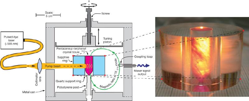
Scientists at NPL chose pentacene doped para-terphenyl instead.
The pentacene has a relatively easily reachable absorption at 585 nm and an intermediate long-lived
decay state with a splitting of 1.45 GHz a long lifetime.
They achieved an output signal of a whooping -10 dBm (100 µW).
Unfortunately, nobody ever picked up on this technique to make an atomic clock.
While I do not think that it would give a good long-term performance (an organic molecule in an other organic
molecule matrix, which would make it very sensitive to changes in environmental conditions and probably have some
strong aging too), the short-term performance could be quite good, due to the strong signal.
One common property of all the atomic clocks mentioned above is, that they use hot atoms.
Meaning, the atoms have a high velocity and move around quite a bit.
This gives rise to a Doppler shift, which depends on the speed of the atomsm and a Doppler broadening,
which depends on the speed distribution of the atoms.
Both lead to a degradation of the performance as the speed cannot be well controlled in many circumstances.
In contrast to this are cold atom standards, which trap the atoms and keep them in confined in a small space.
While some do actually cool the atoms, sometimes to milli-Kelvin temperatures, others keep them
still at room temperature (or even higher), but restrict the movement such, that they are confined
within an area much smaller than the wavelength
(the so called Lamb-Dicke regime),
thus achieving the same effect.
These cold atom clocks can offer much higher long-term stability, as the atoms are even more insulated
from environmental effects, by being kept in the center of a vacuum cavity, not being launched from an oven
or interacting with the walls.
There are two general ways of trapping atoms: neutral atom traps and ion traps.
Neutral atom traps are usually based on magento-optical traps
which traps atoms based on the absorption of laser and its impulse exchange between the absorbed photon and the atom.
This small, but significant impulse pushes the atoms back into the center of the trap.
By applying a magnetic field gradient, it is possible to shift the absorption lines such that only atoms that
are far from the trap center absorb them.
Ion traps use Coulomb repulsion instead.
But, as it is not possible to confine a charged particle in three dimensions by a static field, a changing
field has to be used, which we call a Paul Trap.
The trick is that the field is alternately pushing and pulling, which, together with the atom’s inertia,
gives rise to a virtual potential that, in sum, pushes the atoms towards the center
(also known as the rotating saddle effect).
In this section we will look at two styles of atomic clocks based on neutral traps and ion traps, but
are still based on microwave transitions.
We will look at atomic clocks based on optical transitions in the following section.
As mentioned above, the magento-optical trap (MOT) is the way to cool neutral atoms.
A simplified version of a MOT is an isotropic trap.
Instead of using fibers or mirrors to direct the light from all sides onto the atoms, a reflective
sphere is used.
This way the optics do not need any alignment and just a couple of fibers pointing into the sphere are enough.
This is the idea how the Muquans and Spectradynamics cold rubidium clocks work:
They collect a ball of rubidium in a vacuum chamber in a isotropic trap.
When enough rubidium is collected, they drop the ball and interrogate it with two microwave pulses.
This yields a very high performance atomic clock, which reaches the short-term stability of a passive
hydrogen maser, but without the drift.
The Spectradynamics clock reaches a flicker frequency floor of \(2 \cdot 10^{-15}\).
Even long measurements have not revealed any discernible drift.
These are the clocks I would go for, if I needed a long-term stable clock with good short-term stability.
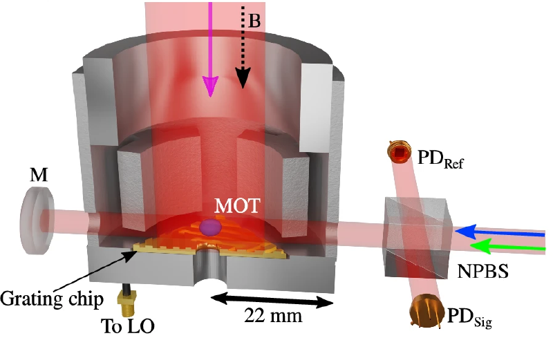
A similar system, using a grating based MOT that drops the rubidium ball only a few millimeters, is in
development in a collaboration between University of Neuchatel and Universtiy of Strathclyde.
The grating allows to relect the light, coming from the top back upwards, but at multiple angles.
This makes it possible to use a single beam to form a complete MOT.
I think this is a very promising technique.
Ions are somewhat easier to trap, as they can be trapped simply by applying a specially crafted
electric field.
Ion traps, have been around since the 1960s and with great success.
Their use in atomic clocks took slightly longer, though.
The earliest example I am aware of was the mercury ion clock developed at HP in the late 70s, early 80s
(see here for an early progress report).
Though, for unknown reason, the work at HP only ever lead to a couple of prototypes being built
and never a series production.
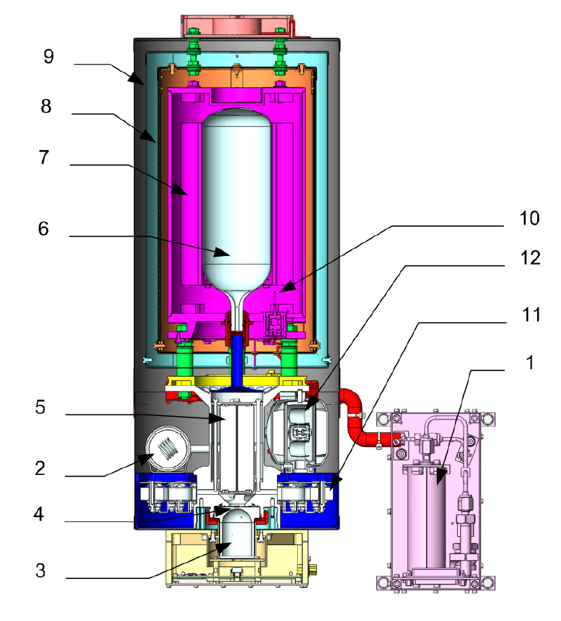
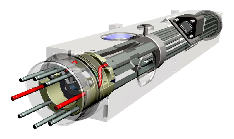
But the idea was later picked up by JPL which developed the deep space atomic clock, whose physics
package you can see above.
Microchip, who eventually bought the remains of the HP atomic clock business, has been developing
a ytterbium based ion microwave standard in recent years.
But the last published performance data was published in
a paper in 2020 and all publications and
slides since, have been using this data.
There are also research groups at universities in the UK and
China working on microwave ion standards (mostly
mercury, ytterbium, and cadmium), but neither of these seem to be mature enough for long-term use.
And these efforts seem to be mostly ignored by the larger scientific community.
Which is, quite honestly, a shame, as microwave ion standards are quite a bit easier to build than
neutral atom microwave clocks, while offering about the same stability.
And what JPL achieved in terms of short-term and
long-term stability is, quite frankly, astounding!
Optical atomic clocks are a rather new thing.
Instead of using atomic transitions with an energy difference that leads to a microwave emission,
they use transitions with large energy differences, that end up in the optical domain.
This has a big immediate advantage: the linewidth, i.e., the uncertainty of the transition’s frequency
for a single measurement, is approximately the same for microwave and optical transitions.
But an optical transition has a four to five orders of magnitude higher frequency.
Which means the relative measurement uncertainty, which is proportional to the linewidth divided
by the transition’s frequency, is four to five orders of magnitude smaller.
I.e. an optical atomic clock is much more accurate and offers, potentially, much lower instability than
a microwave atomic clock.
While optical clocks have been discussed in the 1990s already, and PTB even set out to build one based
on carbon dioxide and later one based on calcium, the big challenge was to relate the optical frequency
to something in the microwave range that could be easily used and measured by electronics.
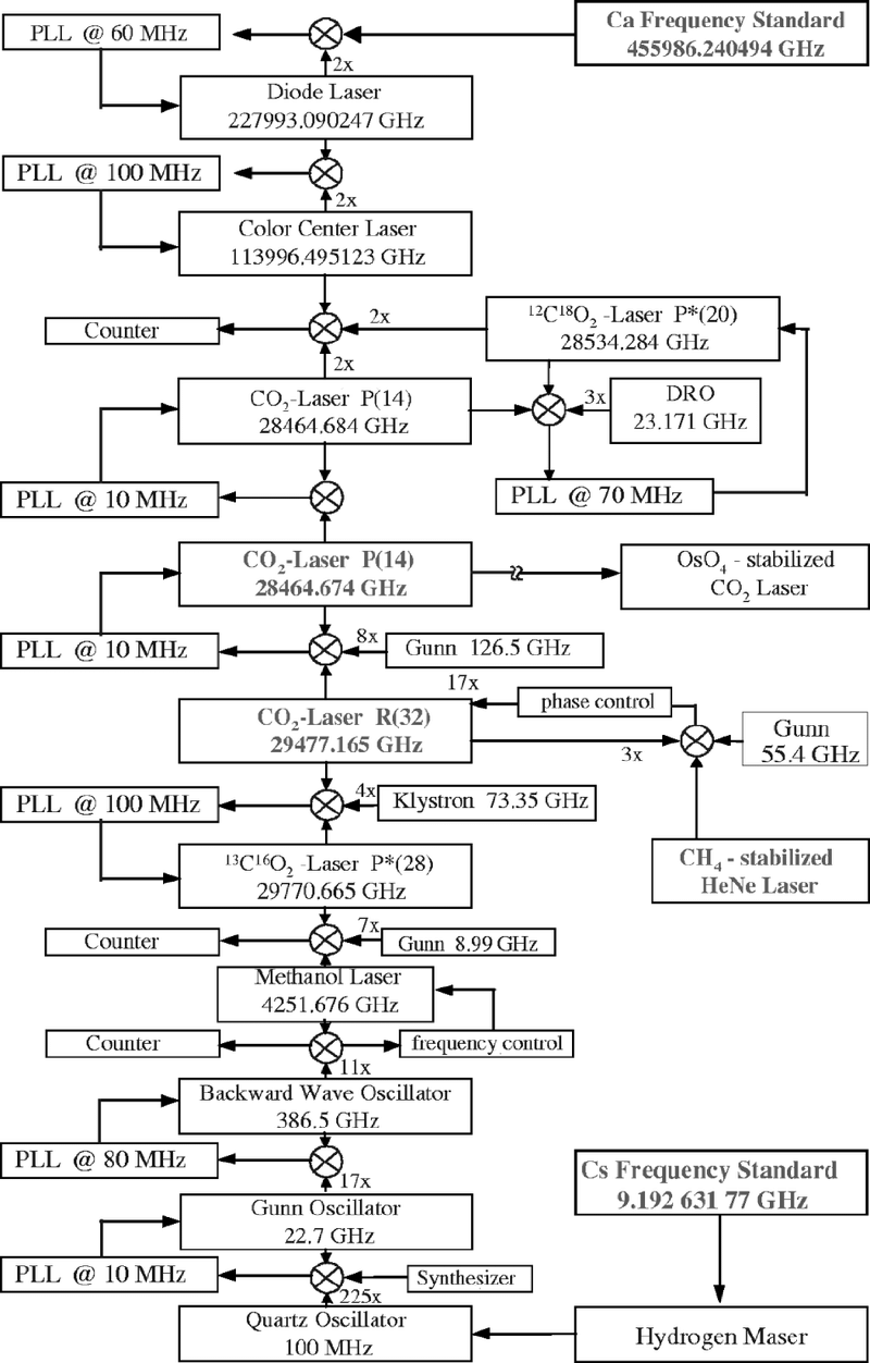
The PTB built an impressive synthesis chain that locked several frequency sources, with ever higher
frequencies, to their microwave clocks.
But using this chain wasn’t easy.
Every measurement took several people many weeks, if not months, to get everything aligned and locked.
It was impractical for a functioning clock.
Though I am impressed they even attempted to do this.
And even more so, they actually managed to get it working!
In the early 2000s, the advent of
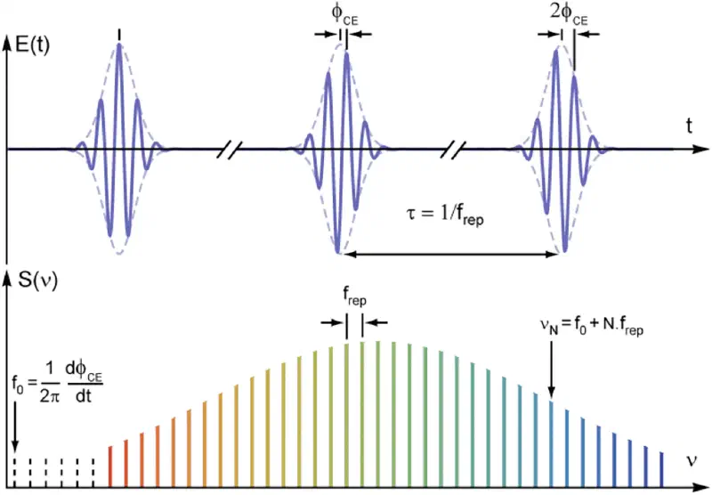
optical frequency combs
(much simplified: fast pulsing lasers with a very stable and well controlled pulsing frequency)
solved this problem (and got the inventors a Nobel price).
These neat little devices allow to divide optical frequencies down to microwave frequencies directly.
This not only allows the direct measurement of optical frequencies, it also divides down any noise
in the optical signal, leading to an unprecedented accuracy!
The first of these frequency combs were rather big and it could take a few hours to get every
piece aligned and the device locked, but today, they are the size of a small shoebox, with even
smaller ones being developed, and can take a beating… well, at least the ones from
Menhir Photonics can.
Once we had a way to easily divide optical frequencies down, the scientific community
dropped everything and started developing optical atomic clocks.
Even though these are very complex devices, there are several laboratories around the
world developing them.
As with cold atom clocks in the microwave domain, there are again two ways to trap atoms:
neutral atom traps and ion traps.
We will have a closer look at both, but quickly review the parts of optical clocks that are
common to both.
As mentioned above, we have an optical frequency comb that relates the optical frequency to a
microwave frequency.
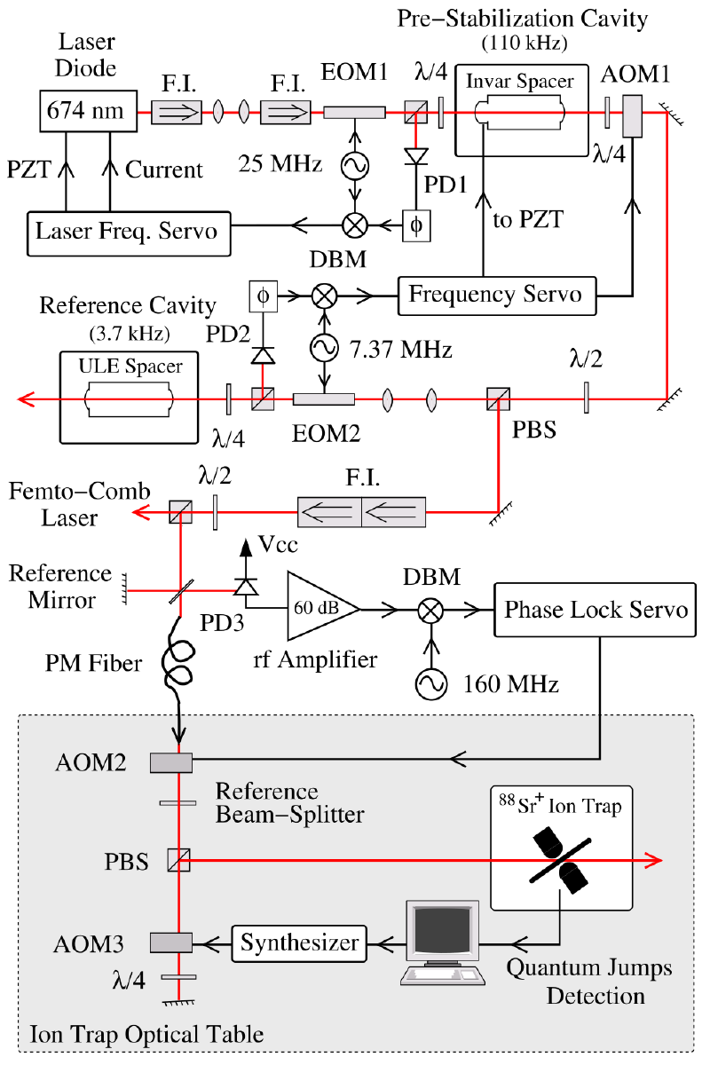
The optical frequency is generated by an optical oscillator, more commonly known as laser.
For reliability reasons he laser used tend to be
external cavity diode lasers (ECDL)
or fiber lasers.
This laser, also called the clock laser, takes the place of the local / fly-wheel oscillator of classic microwave
clocks.
But these lasers are, on their own, not stable enough.
Their short-term frequency fluctuations are rather large, expressed in their linewidth being
several kHz even for the very best lasers, often in the 100s of kHz range.
To stabilize these lasers the common technique is to lock them to a long optical
Fabry-Pérot cavity made from special glass-ceramics
with zero temperature coefficient or a single crystal silicon.
These stabilized lasers reach an ADEV of a few parts in \(10^{-16}\) (around 1 to 10 seconds) with the best
cavities, but even short cavities reach a few parts in \(10^{-15}\) and are regularly around \(10^{-14}\).
Thanks to the optical frequency combs, this translates directly to the stability of the microwave clock.
Of course, this is then rather hard to measure as it means to resolve sub-femtosecond shifts of microwave
signals.
Obviously, reaching these stability values comes at a price.
These cavities’ length has to be stable at \(10^{-16}\) to reach these frequency stabilities.
For a common cavity length of 30cm this means that the length may not fluctuate more than 30am.
That’s 7 orders of magnitude less than the diameter of an atom.
This makes these cavities extremely sensitive to, well, everything.
They are kept in a vibration isolated vacuum chamber with multiple heat shields and
even the laser power entering the cavity has to be stabilized as its heating, or rather the
change in heating, would cause too much fluctuation.
Even people talking near the cavities cause enough vibration to significantly affect the performance of
optical clocks.
I am, quite honestly, amazed that we can reach these stabilities with what is basically a mechanical
device (the length of the cavity).
If someone would have told me, that we would get these values 20 years ago, I would have dismissed it
as wishful thinking and unachievable.
And researchers are still trying to get even better performance out of these cavities!
The development and progress of optical atomic clocks have changed how we do time keeping.
The stability and reliability of these clocks have reached levels where they are now
regularly contributing to TAI,
calibrating the frequency of EAL and thus UTC.
We have even been talking about redefining the second
for some time now.
But, as there is still a lot do to ensure, that the transition to a new definition does not cause
any problems.
So it is unlikely that we see a change in the definition until the CGPM in 2030 or even 2034.
Neutral atoms in microwave clocks are trapped using MOT.
But in optical clocks this does not confine the atoms well enough.
They still move around quite a bit and, more importantly, collide with each other.
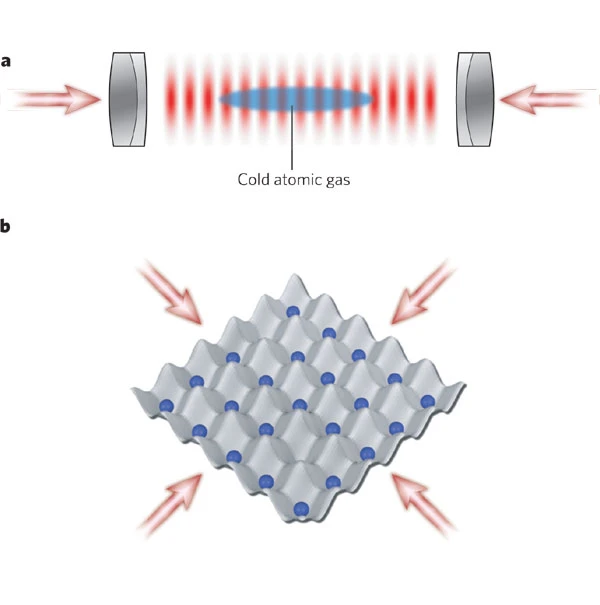
To cool atoms further down and separate them from each other, optical lattices are used, where a strong
laser reflected between mirrors creates a standing wave electromagnetic field, which traps the atoms within
the nodes of this standing wave.
There are certain magic wavelengths, for which the shift induced by the trapping field is zero, thus leading
to a very low disturbance of the atoms.
These optical clocks can trap hundreds to thousands of atoms, thus reaching very high stability values,
even below \(10^{-16}/\sqrt(\tau)\) and have been used to
test general relativity using towers.
(The Katori & Ushijima group/lab at RIKEN is doing some great work.
I recommend checking them out, if you want to know more about optical lattice clocks)
There are already a few national metrology institutes that use optical lattice clocks to calibrate
the frequency of their atomic clock ensembles and to form their local time scale.
Unlike in the microwave case, ion optical clocks mostly trap just a single ion, to have maximum control
over the ion and its environment and thus the least uncertainty over its disturbances.
But because the stability of the clock is then limited by the quantum projection noise, or much simplified: by the number of atoms probed being just one, thus getting a high
statistical uncertainty for determining its state correctly.
Using multiple ions is difficult because even small changes in the electric field caused by the surrounding
ions (i.e., the field experienced is different at the ends vs the center of a group of ions) shift
the optical line up or down by several orders of magnitude of the linewidth itself.
There are techniques to counteract this phenomenon and research projects are underway to explore those,
but we are still at an early stage of this.
Thus, the traps used for optical ion clocks also look different.
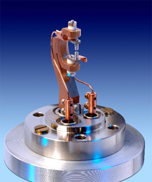
Instead of the linear Paul traps used in microwave ion clocks, the traps in optical ion clocks
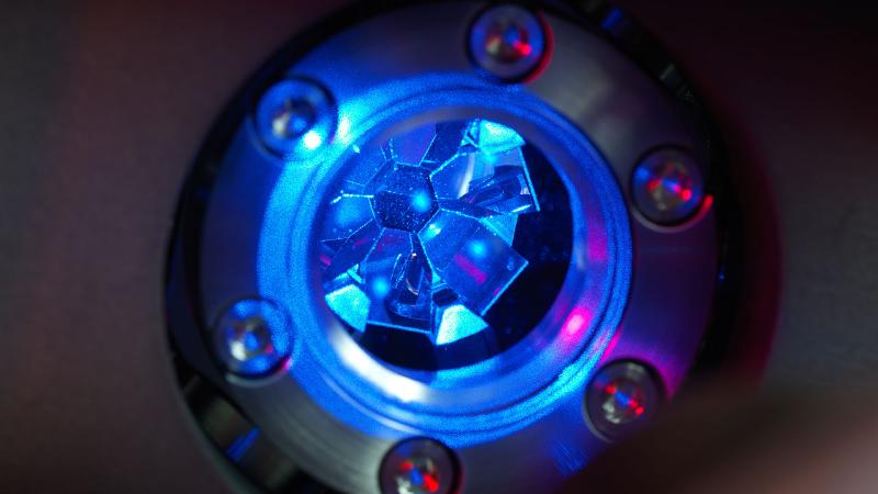
are optimized to give maximum optical access, either by using two stylus like electrodes (endcap trap)
as depicted in the PTB single ion trap above, or by shrinking a linear Paul trap in its z-axis so much it becomes
a plane.
Because a single ion optical clock is severely limited in its short-term stability by the quantum
projection noise limit, ion optical clocks do not deliver the same high short-term to mid-term stability
as optical lattice locks do.
To compensate for this a bit, optical ion clocks tend to try to stabilize the laser better than
lattice clocks, so they can use longer interrogation times, which allows to get a bit better
stability values, though still nowhere near what optical lattice clocks achieve.
But the big advantage of optical ion clocks is their environmental control of the ion.
Because the ion is very well controlled in terms of fields, micro-movement etc, they are the atomic clocks
with the lowest reported uncertainties of below \(10^{-18}\) (see, e.g. the
strontium ion clock developed at VTT Mikes).
A relatively new way to build optical clocks is the so called two photon absorption approach.
Instead of using a narrow transition directly, a phenomenon, where an atom absorbs two photons
to excite a transition is used.
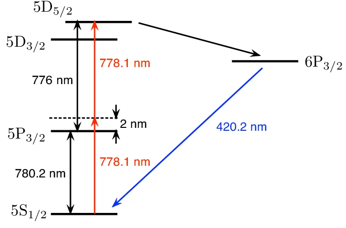
E.g., in the example above for a rubidium 87 atom, there is a high lying \(5D_{5/2}\) energy level,
which would be at a wavelength of 389nm.
As a 389nm laser is rather cumbersome to deal with and not well available, using twice the wavelength (778nm)
is easier and is available as affordable diode lasers.
As can be seen in the level diagram above, the virtual energy level of the two photon absorption is just
above the D1 line, which necessitates some additional care while locking the lasers on the two photon
absorption line.
A big advantage of the two photon absorption scheme is, that a substantial fraction (around 21%)
of the decaying electrons will decay via the \(6P_{3/2}\) level, which gives a fluorescence at 420nm, which is far away from the 778nm laser.
Thus, a simple optical filter makes it possible to isolate the 420nm photons without the strong probe
laser masking the signal.
This makes it possible to continuously probe the transition without the need to switch the probe laser off,
hence giving an additional stability boost.
In total, this gives two photon absorption systems the short-term stability of passive hydrogen masers.
Unfortunately, there is a down-side to this high performance and simplicity.
The first comes from the probe laser being constantly on.
This causes an AC Stark shift, which
is dependent on the laser power.
I.e., any fluctuation of the laser power directly translates to fluctuations in the line’s frequency.
Additionally, because, again for simplicity, two photon absorption systems use small vapor cells,
they are sensitive to changes in environmental conditions (temperature, air pressure).
This leads to a frequency random walk that starts to show up around 1000 to 10'000 seconds and
degrades the long-term performance quite considerably.
This type of frequency standard is still quite new, but there already is some strong commercial interest in it.
I am sure that we will see improvements in short and long-term performance in the coming years.