Simulating Metastability in Digital Circuits Using Spice
Most people probably regard metastability as a solved issue, or rather an issue that barely surfaces. Common wisdom tells us that if you fear that metastability is an issue, then all you need to do is add a synchronizer or wait long enough until it goes away. But when is a synchronizer necessary? And how long is long enough? Measuring metastability is difficult at best in real circuits, more often than not it is impossible to measure directly. Simulation is an alternative, but it is not without problems. Unfortunately there is very little openly documented in on metastability simulation and those few people who know how to do it, are hard to come by. Hence I would like to document here the strategy that worked for me and point at some of the problem one might face.
The Circuit Model
Probably the most important part is to have a good circuit model. At first, this seems to be straight forward and easy to understand, but there are a two big traps. But let's start from the beginning.
Rise/Fall-time of Input
An important factor is how fast your input rises or falls and ultimately, all parameter changes that affect the probability of metastability can be traced back to changes in rise/fall-times of some signal. The rise/fall-time also includes the corners when an input changes, i.e. if the change starts suddenly or smoothly. An example for the former is a spice voltage source which has been programmed to start to rise at some time t. The steepness will go from flat to rising instantaneously. The steepness of the data and clock edge has a large influence on the probability of metastability. Having the wrong rise/fall-time can change the probability by several orders of magnitude easily. Thus you should ensure that the rise time of your signals is correct. It is a good idea, to "filter" the input signals through a chain of inverters in order to make them more "natural."
Transistor Model
The central component of the circuit model is the transistor model. Usually, mismatch between transistor parameters shift the metastable point only up or down a tiny bit, so that is not too critical. But, changes in the capacitance or resistance in a single transistor can shift the probability of metastability up or down by a factor 2 to 3. This means you should use the transistor model you get from the manufacturer, if you have one, instead of a generic one. If you don't have one, then using the Predictive Technology Model parameters is a good start, for exploring, but it should not be mistaken for a real simulation. You will also need to do a sweep through the parameters of different transistors in your circuit to see how much they affect metastability.
Parasitics
Probably the easiest trap to fall into are the parasitics of the circuit. Even though todays transistor models in spice contain all relevant parasitics you will probably face for the transistor, they do not contain the parasitics that arise from the surrounding environment. The interconnect between the transistors and the bulk silicon add quite a bit of capacitance. This capacitance, especially at the nodes with the feedback circuits, are severely affecting metastability and its resolution time. Even a couple of femto-Farad can change your resolution time by a factor of 2 or 3. 10fF, 20fF at the wrong place and your resolution time can change by an order of magnitude, or two. This means, you should be using the post-layout model from your EDA tool whenever possible.
Numerical Precision
As the simulation will be dealing with minuscule changes of voltages, it is important that the numerical precision is high. Most simulation tools do not allow to change the numerical representation of the voltages and currents, which gives a lower limit how precisely metastability can be modeled. Another important issue is the size of the time steps. These have to small enough to not introduce any significant error in the calculations. And the closer the simulation gets to the metastable point, the smaller the maximum time step has to be. As a rule of thumb, choose the maximum size smaller than one tenth of the distance to the metastable point.
Simulating
Simulation of metastability will almost always have two steps: first estimating where the metastable point is, then doing the simulation with the right parameters.
The metastable point estimation can be done using a transient simulation with relatively crude time steps (i.e. a fast simulation) and is just a binary search where metastability happens. I.e. choose two values for the delay between data input and clock. One such that the output does not change and a second such that the output does change. Then half the time, simulate and see to which value the output stabilizes. Replace the upper or lower value accordingly and repeat. Once you have found the metastable point with sufficient accuracy (i.e. the distance between the upper and the lower delay is small enough) you are done.
The smaller the distance is, the smaller the time steps of your simulation should become. But be aware that you might accidentally just hit the metastable point and your simulation might output might be wrong due to inaccuracies. Hence it is a good idea to rerun the simulation in a narrow range around the metastable point you just determined, with full precision, to ensure that you got it right.
After you know where the metastable point is, you can run the simulation to generate the data you really want. Start again with an upper (or lower) delay value and use the estimated metastable point as the second one. With each simulation you record the time it takes for the voltages to reach their stable values. For each step you half the time time between the upper (or lower) and the metastable point and replace the upper (or lower) point.
If you have set your simulation parameters correctly, you will see something like this:
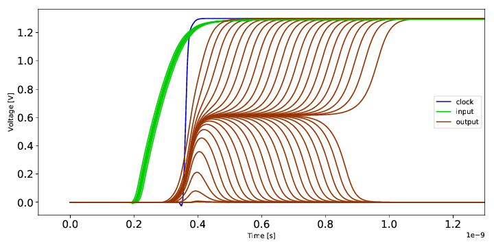
As you can see, a very small change of the data input timing (the thick and blurry green line), relative to the clock edge (in blue), has a large influence on the output (the curves in red). Especially note that the length of the metastability, where the output is stuck in between logic levels, can be arbitrary long and the resolution can go to one side or the other with equal probability. The limit in simulation is the numerical precision, as at some point the simulation output becomes unstable.
From the recorded data, you can now plot how much the stabilization time changes, with the time distance between data input and clock input:
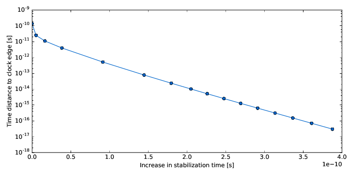
Note that the data to clock delay has been normalized such that 0 is the metastable point. From this data you can calculate the time constant of the stabilization and the critical window size, if you wish to.
- Attila Kinali's blog
- Log in to post comments